"Web prototype": the code on this page is a JavaScript study; Islands does not have it yet.«Prototipo web»: el código de esta página es un estudio en JavaScript; Islands todavía no lo tiene.
Spreading Points on a Plane
Trees, rocks and towns on a map need points that look random but never too close. Here are eight ways to spread them, measured with the same numbers. Tap a thumbnail, look at the highlighted pairs and the seams between chunks, and press ▶ to see the order in which each method places them.✦ IA How it works.
Árboles, rocas y pueblos en un mapa necesitan puntos que parezcan al azar, pero nunca demasiado juntos. Aquí hay ocho maneras de repartirlos, medidas con los mismos números. Toca una viñeta, mira los pares resaltados y las costuras entre chunks, y pulsa ▶ para ver en qué orden los coloca cada método.✦ IA Cómo funciona.
The idea in plain words
Scatter points at random and you get clumps and holes; line them up and the grid shows. A procedural world usually wants something in between: random, but never too close. Graphics calls it blue noise.
Each method tries in its own way. Bridson sows with a hand's width of room round every point; hashed priority runs a lottery per cell where only the best number in the neighbourhood stays; Lloyd pushes the points like soap bubbles until they are even. Look at the highlighted pairs, the dashed circle and the seams. ✦ IA
Why it matters
A world generator places trees, rocks and towns, and nearly always wants that "never too close". Nature got there first: the cones of the macaque retina are spread this way (Yellott 1983), Cook (1986) brought the idea to image sampling, and Matérn (1960) modelled it for the trees of Swedish forests. ✦ IA
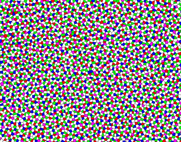

For Islands one more thing matters: the world is built in chunks as the player walks. A method that depends on order, like Bridson, leaves seams; one that comes from the hash, like priority, does not. ✦ IA
Is there a theorem?
Two results explain the table. Priority with one round is Matérn's type II process, which never exceeds 1/(πr²) points per unit of area, while dropping discs at random until none fits covers about 54.7 % of the plane (Feder 1980): hence half as many points as Bridson. The rounds follow Luby's idea (1986) and, with enough of them, reach the set where no candidate fits any more. ✦ IA
The equations
r = √(0.65 / n) (Bridson gives about n points per unit of area with this r; measured)
φb(i) = Σ dk b−k−1, with i = Σ dk bk (Halton: point i = (φ2(i), φ3(i)))
λII = (1 − e−λπr²) / (πr²) < 1 / (πr²) (Matérn II density from λ candidates)
P(k) = |Σj e−2πi k·xj|² / n (spectrum; uniform random gives 1 at every frequency)
What the numbers say
Bridson has the best closest pair (0.81), but computed by chunks it leaves about 50 pairs too close at the seams. Hashed priority leaves none and gives exactly the same by chunks as whole; with one round it loses half the points, with three it keeps 77 %. Sobol' and Halton are the most even at large scale and Lloyd the most regular up close, but none of them works by chunks. For Islands' trees, the candidate is hashed priority with three rounds. ✦ IA
What the picture does and does not show ✦ IA
- Discs have diameter r, the same r for every method: two overlapping discs are a pair closer than r. For Halton, Sobol', random and Lloyd, r is not part of the method; it is a yardstick.
- The spectrum is the mean of 8 seeds. One alone is too noisy to show the ring.
- The largest gap and Lloyd are measured on a raster of samples (96, and up to 320 a side), not exactly: they are accurate to about one sample.
- The edges of the square count. Bridson and Lloyd cannot see past them, hashed priority can (its candidates carry on outside), so the edges look different.
- The llareta is a first approach: rosettes as discs with five tips, in three greens by light, with no checked data on rosette size.
All together: a sea of points
In Sea of Points hashed priority spreads an endless map, with r varying along a noise field and regions using different methods, with no seams between chunks or between regions. And in the Araucaria Forest each point becomes a tree whose age sets its r. ✦ IA
How it works ✦ IA
This part walks through the scene's code, step by step. It covers:
- Repeatable random numbers per cell, with the hash of part 1.
- The jittered grid, as Islands uses it.
- Halton and Sobol': mirroring digits and mixing bits.
- Bridson's Poisson disk, and why it depends on order.
- Hashed-priority Poisson disk, in rounds.
- Lloyd relaxation on a raster of samples.
- Three measures: neighbours, spectrum and the seam test.
Plain JavaScript and the Canvas 2D API, no libraries. Point sets are flat lists
[x0, y0, x1, y1, …], to move to C# without objects.
1. One random number per cell
As in part 5, but with two coordinates: the hash takes the seed, the column, the row and a salt per use. Any cell can then be computed alone, in any order.
// A uniform number in [0, 1) from (seed, a, b, salt). Full 32 bits.
export function h01(s, a, b, salt) {
  return avalanche(eat(eat(eat(seed(s), a), b), salt)) / TWO32;
}
2. The jittered grid
One point per cell of a global grid of step 1/√n, anywhere in its cell. Because a cell is named by its integer coordinates, a chunk computed alone gets exactly the points of the whole world.
// One point per cell of a global lattice of step `cell`, anywhere inside it. The cell
// is hashed by its integer coordinates, as in Noise.Voronoi, so a chunk computed alone
// gets exactly the points of the whole.
export function jittered(cell, s, b = UNIT) {
  const out = [];
  const i0 = Math.floor(b.x0 / cell), i1 = Math.ceil(b.x1 / cell);
  const j0 = Math.floor(b.y0 / cell), j1 = Math.ceil(b.y1 / cell);
  for (let j = j0; j < j1; j++) {
    for (let i = i0; i < i1; i++) {
      const x = (i + h01(s, i, j, 2)) * cell, y = (j + h01(s, i, j, 3)) * cell;
      if (inside(x, y, b)) out.push(x, y);
    }
  }
  return out;
}
3. Halton and Sobol'
Halton writes the index in base 2 for x and in base 3 for y, and mirrors the digits about the point. The seed shifts the whole set on the torus (Cranley and Patterson).
// Radical inverse in any base: mirror the digits of i about the point.
export function radicalInverse(i, base) {
  let r = 0, f = 1 / base;
  for (; i > 0; i = Math.floor(i / base), f /= base) r += (i % base) * f;
  return r;
}

// Halton (bases 2 and 3), shifted on the torus by the seed (Cranley–Patterson).
out.push(b.x0 + w * frac(radicalInverse(i, 2) + sx),
         b.y0 + h * frac(radicalInverse(i, 3) + sy));
Sobol' uses base 2 on both axes, but mixes the bits of y with "direction numbers" from a polynomial; for the second axis, x + 1 is enough. The seed XORs a hashed word, which keeps the structure.
// Dimension 2: primitive polynomial x + 1, m_k = 2·m_(k−1) XOR m_(k−1), m_1 = 1.
const SOBOL_V2 = (() => {
  const v = new Uint32Array(32);
  let m = 1;
  for (let k = 1; k <= 32; k++) {
    v[k - 1] = (m << (32 - k)) >>> 0;
    m = (m << 1) ^ m;
  }
  return v;
})();

// Point i: XOR the direction numbers of the bits that are set in i.
for (let k = 0, bits = i; bits; k++, bits >>>= 1) {
  if (bits & 1) { x ^= 0x80000000 >>> k; y ^= SOBOL_V2[k]; }
}
// The seed XORs both with a hashed word: a random digital shift.
out.push(((x ^ dx) >>> 0) / TWO32, ((y ^ dy) >>> 0) / TWO32);
4. Bridson
A list of active points. Pick one at random and try up to k = 30 candidates in the ring between r and 2r. The first one at least r from everyone joins and becomes active; if none fits, the point retires. A grid of step r/√2 holds one point per cell, so checking a candidate only looks at 5 × 5 cells.
add(randomPointInBox());
while (active.length) {
  const a = Math.floor(rnd() * active.length), p = active[a];
  let placed = false;
  for (let t = 0; t < k && !placed; t++) {
    // A candidate in the ring between r and 2r.
    const ang = 2 * Math.PI * rnd(), d = r * (1 + rnd());
    const x = pts[2 * p] + d * Math.cos(ang), y = pts[2 * p + 1] + d * Math.sin(ang);
    if (inside(x, y, b) && fits(x, y)) { add(x, y); placed = true; }
  }
  if (!placed) { active[a] = active[active.length - 1]; active.pop(); }   // no room around p
}
Every point depends on those that came before. Two chunks computed apart know nothing of each other, and their points clash at the seam: the red pairs in the third figure.
5. Hashed priority, in rounds
One candidate per cell of step r/√2, moved by the hash, with a priority that also comes from the hash. In each round, every undecided candidate that no undecided neighbour within r outranks joins, and its neighbours drop out. One round is Matérn's type II process; more rounds give another chance to whoever lost to someone who then did not join either (Luby).
for (let t = 1; t <= rounds; t++) {
  const join = [];
  for (let c = 0; c < n; c++) {
    if (state[c] !== 0) continue;                 // already in or out
    let wins = true;
    each(c, (o) => { if (wins && state[o] === 0 && beats(o, c)) wins = false; });
    if (wins) join.push(c);                       // no undecided neighbour outranks it
  }
  if (!join.length) break;
  for (const c of join) state[c] = 1;
  for (const c of join) each(c, (o) => { if (state[o] === 0) state[o] = -1; });
}
Each round only looks 2r away. With a border that wide per round, a chunk gives the same as the whole world, and the scene checks it: "Same as the whole square: yes".
// A point inside b depends only on candidates within 2r per round, so a halo of that
// width makes a chunk computed alone equal to the whole: no order, no seams.
const cell = r / Math.SQRT2, halo = Math.ceil((2 * r * rounds) / cell) + 1;
6. Lloyd
Every point moves to the centre of its Voronoi cell. Instead of building the diagram, a raster of samples is shared out: each sample goes to its nearest point, and each cell's centre is the mean of its samples. Slow (about 40 ms for 20 steps at 256 points) and global.
for (let it = 0; it < steps; it++) {
  const g = buckets(pts, Math.sqrt((w * h) / n), b);
  sx.fill(0); sy.fill(0); cnt.fill(0);
  for (let j = 0; j < side; j++) {
    for (let i = 0; i < side; i++) {
      const px = b.x0 + ((i + 0.5) / side) * w, py = b.y0 + ((j + 0.5) / side) * h;
      const { p } = nearest(pts, g, px, py);      // the sample belongs to p's cell
      sx[p] += px; sy[p] += py; cnt[p]++;
    }
  }
  for (let p = 0; p < n; p++) if (cnt[p]) { pts[2 * p] = sx[p] / cnt[p]; pts[2 * p + 1] = sy[p] / cnt[p]; }
}
7. Measuring: neighbours, spectrum and seams
Distances are found with a grid of buckets, ring by ring, until no farther point can win. The spectrum adds one wave per point and frequency; since a 2D wave is the product of one per axis, one row of powers per axis is enough.
// P(k) = |Σ exp(−2πi k·x)|² / n. Separable: one row of powers per axis and point.
for (let p = 0; p < n; p++) {
  powers(pts[2 * p], K, ex);
  powers(pts[2 * p + 1], K, ey);
  for (let v = 0; v < side; v++) {
    const yr = ey[2 * v], yi = ey[2 * v + 1], row = v * side;
    for (let u = 0; u < side; u++) {
      const xr = ex[2 * u], xi = ex[2 * u + 1];
      re[row + u] += xr * yr - xi * yi;
      im[row + u] += xr * yi + xi * yr;
    }
  }
}
The seam test cuts the square into 3 × 3 chunks, computes each one alone and compares the result with the whole square.
export function chunked(m, n, s, k, opts = {}, whole = null) {
  const pts = [], chunkOf = [];
  for (let cj = 0; cj < k; cj++) {
    for (let ci = 0; ci < k; ci++) {
      const b = { x0: ci / k, y0: cj / k, x1: (ci + 1) / k, y1: (cj + 1) / k };
      const part = m.make(n, s, b, opts);
      for (let q = 0; q < part.length; q += 2) { pts.push(part[q], part[q + 1]); chunkOf.push(cj * k + ci); }
    }
  }
  const all = whole || m.make(n, s, UNIT, opts);
  return { pts, chunkOf, sameAsWhole: sameSet(pts, all) };
}
A note for Islands ✦ IA
Islands only has the jittered grid (inside Noise.Voronoi), and its
MapContext2D carries a sequential ctx.Rng (checked 2026-10-28).
Hashed priority meets the three conditions of the design note: deterministic, parallel per
cell and seam-free, with a border of about 3 cells per round. With 3 rounds it gives 77 % of
Bridson's points (199 against 260) and no conflict at the seams; with 3 candidates per cell, 85 % (222). Results in
Documentation~/research/points-2d-results.md.
Going further
Wei (2008) does Poisson disk in parallel by groups of cells, and Lagae and Dutré (2008) compare a dozen methods with one measure. Owen (1995) scrambles Sobol' without losing its properties. Voronoi, the next thing done with these points, is part 7. ✦ IA
La idea en palabras sencillas
Si repartes puntos al azar, salen grumos y claros; si los alineas, se nota la rejilla. Un mundo procedural suele querer algo intermedio: al azar, pero nunca demasiado cerca. En gráficos se llama ruido azul.
Cada método lo intenta a su manera. Bridson siembra dejando un palmo libre alrededor de cada punto; la prioridad con hash hace una lotería por celda en la que solo se queda el mejor número del barrio; Lloyd empuja los puntos como burbujas de jabón hasta que quedan parejos. Mira los pares resaltados, el círculo discontinuo y las costuras. ✦ IA
Por qué importa
Un generador de mundos coloca árboles, rocas y pueblos, y casi siempre quiere ese «nunca demasiado cerca». La naturaleza llegó antes: los conos de la retina del macaco se reparten así (Yellott 1983), Cook (1986) llevó la idea al muestreo de imágenes y Matérn (1960) la modeló para los árboles de los bosques suecos. ✦ IA
Para Islands importa algo más: el mundo se genera por chunks mientras el jugador camina. Un método que depende del orden, como Bridson, deja costuras; uno que sale del hash, como la prioridad, no. ✦ IA
¿Hay un teorema?
Dos resultados explican la tabla. La prioridad con una ronda es el proceso de Matérn de tipo II, que nunca pasa de 1/(πr²) puntos por unidad de área, mientras que dejar caer discos al azar hasta que no cabe ninguno llena cerca del 54,7 % del plano (Feder 1980): por eso salen la mitad de puntos que con Bridson. Las rondas siguen la idea de Luby (1986) y, con las suficientes, llegan al conjunto en el que ya no cabe ningún candidato más. ✦ IA
Las ecuaciones
r = √(0,65 / n) (Bridson da unos n puntos por unidad de área con este r; medido)
φb(i) = Σ dk b−k−1, con i = Σ dk bk (Halton: punto i = (φ2(i), φ3(i)))
λII = (1 − e−λπr²) / (πr²) < 1 / (πr²) (densidad de Matérn II a partir de λ candidatos)
P(k) = |Σj e−2πi k·xj|² / n (espectro; el azar uniforme da 1 en todas las frecuencias)
Qué dicen los números
Bridson tiene la mejor distancia mínima (0,81), pero calculado por chunks deja unos 50 pares demasiado cerca en las costuras. La prioridad con hash no deja ninguno y por trozos da exactamente lo mismo que entero; con una ronda pierde la mitad de los puntos y con tres conserva el 77 %. Sobol' y Halton son los más parejos a gran escala y Lloyd el más regular de cerca, pero ninguno sirve por chunks. Para los árboles de Islands, el candidato es la prioridad con hash y tres rondas. ✦ IA
Qué dice y qué no dice la imagen ✦ IA
- Los discos miden r de diámetro, el mismo r para todos los métodos: dos discos que se solapan son un par a menos de r. Para Halton, Sobol', el azar y Lloyd, r no forma parte del método; es una vara para comparar.
- El espectro es la media de 8 semillas. Una sola es demasiado ruidosa para ver el anillo.
- El hueco mayor y Lloyd se miden en una rejilla de muestras (96 y hasta 320 por lado), no de forma exacta: son aproximaciones del orden de una muestra.
- Los bordes del cuadrado cuentan. Bridson y Lloyd no ven fuera, la prioridad con hash sí (sus candidatos siguen más allá), y por eso los bordes se ven distintos.
- La llareta es un primer acercamiento: rosetas como discos con cinco puntas, en tres verdes según la luz, sin datos de tamaño de roseta verificados.
Todo junto: un mar de puntos
En Mar de puntos la prioridad con hash reparte un mapa que no termina, con r variable según un campo de ruido y regiones con métodos distintos, sin costuras entre chunks ni entre regiones. Y en el Bosque de araucarias cada punto pasa a ser un árbol cuya edad fija su r. ✦ IA
Cómo funciona ✦ IA
Esta parte recorre el código de la escena, paso a paso. Cubre:
- Números aleatorios repetibles por celda, con el hash de la parte 1.
- La rejilla con jitter, como la usa Islands.
- Halton y Sobol': dar la vuelta a las cifras y mezclar bits.
- El disco de Poisson de Bridson, y por qué depende del orden.
- El disco de Poisson por prioridad con hash, en rondas.
- La relajación de Lloyd sobre una rejilla de muestras.
- Tres medidas: vecinos, espectro y la prueba de costuras.
JavaScript sin más y la API Canvas 2D, sin librerías. Los conjuntos de puntos son listas
planas [x0, y0, x1, y1, …], para pasarlos a C# sin objetos. Los comentarios del
código están en inglés.
1. Un número aleatorio por celda
Igual que en la parte 5, pero con dos coordenadas: el hash recibe la semilla, la columna, la fila y una sal por uso. Así cualquier celda se puede calcular sola, en cualquier orden.
// A uniform number in [0, 1) from (seed, a, b, salt). Full 32 bits.
export function h01(s, a, b, salt) {
  return avalanche(eat(eat(eat(seed(s), a), b), salt)) / TWO32;
}
2. La rejilla con jitter
Un punto por celda de una rejilla global de paso 1/√n, en cualquier sitio de su celda. Como la celda se identifica por sus coordenadas enteras, un chunk calculado solo da exactamente los mismos puntos que el mundo entero.
// One point per cell of a global lattice of step `cell`, anywhere inside it. The cell
// is hashed by its integer coordinates, as in Noise.Voronoi, so a chunk computed alone
// gets exactly the points of the whole.
export function jittered(cell, s, b = UNIT) {
  const out = [];
  const i0 = Math.floor(b.x0 / cell), i1 = Math.ceil(b.x1 / cell);
  const j0 = Math.floor(b.y0 / cell), j1 = Math.ceil(b.y1 / cell);
  for (let j = j0; j < j1; j++) {
    for (let i = i0; i < i1; i++) {
      const x = (i + h01(s, i, j, 2)) * cell, y = (j + h01(s, i, j, 3)) * cell;
      if (inside(x, y, b)) out.push(x, y);
    }
  }
  return out;
}
3. Halton y Sobol'
Halton escribe el índice en base 2 para x y en base 3 para y, y les da la vuelta a las cifras alrededor de la coma. La semilla desplaza todo el conjunto sobre el toro (Cranley y Patterson).
// Radical inverse in any base: mirror the digits of i about the point.
export function radicalInverse(i, base) {
  let r = 0, f = 1 / base;
  for (; i > 0; i = Math.floor(i / base), f /= base) r += (i % base) * f;
  return r;
}

// Halton (bases 2 and 3), shifted on the torus by the seed (Cranley–Patterson).
out.push(b.x0 + w * frac(radicalInverse(i, 2) + sx),
         b.y0 + h * frac(radicalInverse(i, 3) + sy));
Sobol' usa base 2 en los dos ejes, pero en y mezcla los bits con unos «números de dirección» que salen de un polinomio. Para el segundo eje basta con el polinomio x + 1. La semilla hace un XOR con una palabra del hash, que conserva la estructura.
// Dimension 2: primitive polynomial x + 1, m_k = 2·m_(k−1) XOR m_(k−1), m_1 = 1.
const SOBOL_V2 = (() => {
  const v = new Uint32Array(32);
  let m = 1;
  for (let k = 1; k <= 32; k++) {
    v[k - 1] = (m << (32 - k)) >>> 0;
    m = (m << 1) ^ m;
  }
  return v;
})();

// Point i: XOR the direction numbers of the bits that are set in i.
for (let k = 0, bits = i; bits; k++, bits >>>= 1) {
  if (bits & 1) { x ^= 0x80000000 >>> k; y ^= SOBOL_V2[k]; }
}
// The seed XORs both with a hashed word: a random digital shift.
out.push(((x ^ dx) >>> 0) / TWO32, ((y ^ dy) >>> 0) / TWO32);
4. Bridson
Una lista de puntos activos. Se elige uno al azar y se prueban hasta k = 30 candidatos en el anillo entre r y 2r. El primero que queda a r o más de todos entra y se vuelve activo; si ninguno cabe, el punto se retira. Una rejilla de paso r/√2 guarda un punto por celda, así que comprobar un candidato solo mira 5 × 5 celdas.
add(randomPointInBox());
while (active.length) {
  const a = Math.floor(rnd() * active.length), p = active[a];
  let placed = false;
  for (let t = 0; t < k && !placed; t++) {
    // A candidate in the ring between r and 2r.
    const ang = 2 * Math.PI * rnd(), d = r * (1 + rnd());
    const x = pts[2 * p] + d * Math.cos(ang), y = pts[2 * p + 1] + d * Math.sin(ang);
    if (inside(x, y, b) && fits(x, y)) { add(x, y); placed = true; }
  }
  if (!placed) { active[a] = active[active.length - 1]; active.pop(); }   // no room around p
}
Cada punto depende de los que entraron antes. Dos chunks calculados por separado no saben nada el uno del otro, y sus puntos chocan en la costura: los pares rojos de la tercera figura.
5. Prioridad con hash, en rondas
Un candidato por celda de paso r/√2, desplazado por el hash, con una prioridad que también sale del hash. En cada ronda entra todo candidato sin decidir al que no supera ningún vecino sin decidir a menos de r, y sus vecinos quedan fuera. Una ronda es el proceso de Matérn de tipo II; más rondas dan otra oportunidad a quien perdió frente a alguien que luego tampoco entró (Luby).
for (let t = 1; t <= rounds; t++) {
  const join = [];
  for (let c = 0; c < n; c++) {
    if (state[c] !== 0) continue;                 // already in or out
    let wins = true;
    each(c, (o) => { if (wins && state[o] === 0 && beats(o, c)) wins = false; });
    if (wins) join.push(c);                       // no undecided neighbour outranks it
  }
  if (!join.length) break;
  for (const c of join) state[c] = 1;
  for (const c of join) each(c, (o) => { if (state[o] === 0) state[o] = -1; });
}
Cada ronda solo mira a 2r de distancia. Con un borde de ese ancho por ronda, un chunk da lo mismo que el mundo entero, y la escena lo comprueba: «Igual al cuadrado entero: sí».
// A point inside b depends only on candidates within 2r per round, so a halo of that
// width makes a chunk computed alone equal to the whole: no order, no seams.
const cell = r / Math.SQRT2, halo = Math.ceil((2 * r * rounds) / cell) + 1;
6. Lloyd
Cada punto se muda al centro de su celda de Voronoi. En vez de construir el diagrama, se reparte una rejilla de muestras: cada muestra va al punto más cercano, y el centro de cada celda es la media de sus muestras. Es lento (unos 40 ms por 20 pasos a 256 puntos) y global.
for (let it = 0; it < steps; it++) {
  const g = buckets(pts, Math.sqrt((w * h) / n), b);
  sx.fill(0); sy.fill(0); cnt.fill(0);
  for (let j = 0; j < side; j++) {
    for (let i = 0; i < side; i++) {
      const px = b.x0 + ((i + 0.5) / side) * w, py = b.y0 + ((j + 0.5) / side) * h;
      const { p } = nearest(pts, g, px, py);      // the sample belongs to p's cell
      sx[p] += px; sy[p] += py; cnt[p]++;
    }
  }
  for (let p = 0; p < n; p++) if (cnt[p]) { pts[2 * p] = sx[p] / cnt[p]; pts[2 * p + 1] = sy[p] / cnt[p]; }
}
7. Medir: vecinos, espectro y costuras
Las distancias se buscan con una rejilla de cubetas, anillo a anillo, hasta que ningún punto más lejano puede ganar. El espectro suma una onda por punto y frecuencia; como la onda en 2D es el producto de una por eje, basta con una fila de potencias por eje.
// P(k) = |Σ exp(−2πi k·x)|² / n. Separable: one row of powers per axis and point.
for (let p = 0; p < n; p++) {
  powers(pts[2 * p], K, ex);
  powers(pts[2 * p + 1], K, ey);
  for (let v = 0; v < side; v++) {
    const yr = ey[2 * v], yi = ey[2 * v + 1], row = v * side;
    for (let u = 0; u < side; u++) {
      const xr = ex[2 * u], xi = ex[2 * u + 1];
      re[row + u] += xr * yr - xi * yi;
      im[row + u] += xr * yi + xi * yr;
    }
  }
}
La prueba de costuras corta el cuadrado en 3 × 3 chunks, calcula cada uno solo y compara el resultado con el cuadrado entero.
export function chunked(m, n, s, k, opts = {}, whole = null) {
  const pts = [], chunkOf = [];
  for (let cj = 0; cj < k; cj++) {
    for (let ci = 0; ci < k; ci++) {
      const b = { x0: ci / k, y0: cj / k, x1: (ci + 1) / k, y1: (cj + 1) / k };
      const part = m.make(n, s, b, opts);
      for (let q = 0; q < part.length; q += 2) { pts.push(part[q], part[q + 1]); chunkOf.push(cj * k + ci); }
    }
  }
  const all = whole || m.make(n, s, UNIT, opts);
  return { pts, chunkOf, sameAsWhole: sameSet(pts, all) };
}
Una nota para Islands ✦ IA
Islands solo tiene la rejilla con jitter (dentro de Noise.Voronoi), y su
MapContext2D lleva un ctx.Rng secuencial (comprobado el 2026-10-28).
La prioridad con hash cumple las tres condiciones de la nota de diseño: determinista, paralela
por celda y sin costuras, con un borde de unas 3 celdas por ronda. Con 3 rondas da el 77 % de
los puntos de Bridson (199 frente a 260) y ningún conflicto en las costuras; con 3 candidatos por celda, el 85 % (222). Resultados en
Documentation~/research/points-2d-results.md.
Para ir más allá
Wei (2008) hace el disco de Poisson en paralelo por grupos de celdas, y Lagae y Dutré (2008) comparan una docena de métodos con una misma medida. Owen (1995) desordena Sobol' sin perder sus propiedades. Voronoi, lo siguiente que se hace con estos puntos, es la parte 7. ✦ IA
SourcesFuentes
- R. L. Cook, "Stochastic sampling in computer graphics", ACM Trans. Graph. 5(1) (1986) 51–72. Jittered sampling and dart throwing. doi.org/10.1145/7529.8927
- J. I. Yellott, "Spectral consequences of photoreceptor sampling in the rhesus retina", Science 221 (1983) 382–385. doi.org/10.1126/science.6867716
- R. Ulichney, Digital Halftoning, MIT Press (1987). Where "blue noise" is named.
- R. Bridson, "Fast Poisson disk sampling in arbitrary dimensions", SIGGRAPH 2007 Sketches, article 22. doi.org/10.1145/1278780.1278807
- B. Matérn, Spatial Variation, 2nd ed., Lecture Notes in Statistics 36, Springer (1986). First published 1960 by the Swedish forest research institute; the hard-core processes. doi.org/10.1007/978-1-4615-7892-5
- Y. Jiao, T. Lau, H. Hatzikirou, M. Meyer-Hermann, J. C. Corbo, S. Torquato, "Avian photoreceptor patterns represent a disordered hyperuniform solution to a multiscale packing problem", Phys. Rev. E 89 (2014) 022721. doi.org/10.1103/PhysRevE.89.022721
- M. Luby, "A simple parallel algorithm for the maximal independent set problem", SIAM J. Comput. 15(4) (1986) 1036–1053. doi.org/10.1137/0215074
- J. Feder, "Random sequential adsorption", J. Theor. Biol. 87(2) (1980) 237–254. Discs dropped at random until none fits cover about 54.7 % of the plane. doi.org/10.1016/0022-5193(80)90358-6
- L.-Y. Wei, "Parallel Poisson disk sampling", ACM Trans. Graph. 27(3) (2008), article 20. doi.org/10.1145/1360612.1360619
- A. Lagae, P. Dutré, "A comparison of methods for generating Poisson disk distributions", Computer Graphics Forum 27(1) (2008) 114–129. doi.org/10.1111/j.1467-8659.2007.01100.x
- J. H. Halton, "On the efficiency of certain quasi-random sequences of points in evaluating multi-dimensional integrals", Numerische Mathematik 2 (1960) 84–90. doi.org/10.1007/BF01386213
- I. M. Sobol', "On the distribution of points in a cube and the approximate evaluation of integrals", USSR Comput. Math. Math. Phys. 7(4) (1967) 86–112. doi.org/10.1016/0041-5553(67)90144-9
- R. Cranley, T. N. L. Patterson, "Randomization of number theoretic methods for multiple integration", SIAM J. Numer. Anal. 13(6) (1976) 904–914. doi.org/10.1137/0713071
- S. Paskov, J. Traub, "Faster valuation of financial derivatives", J. Portfolio Management 22(1) (1995) 113–120. Sobol' points beat Monte Carlo on a mortgage-backed bond. doi.org/10.3905/jpm.1995.409541
- S. P. Lloyd, "Least squares quantization in PCM", IEEE Trans. Inf. Theory 28(2) (1982) 129–137. doi.org/10.1109/TIT.1982.1056489
- Q. Du, V. Faber, M. Gunzburger, "Centroidal Voronoi tessellations: applications and algorithms", SIAM Review 41(4) (1999) 637–676. doi.org/10.1137/S0036144599352836
- A. Secord, "Weighted Voronoi stippling", NPAR 2002, 37–43. doi.org/10.1145/508530.508537
- S. Worley, "A cellular texture basis function", SIGGRAPH '96, 291–294. doi.org/10.1145/237170.237267
- A. Patel, "Polygonal map generation for games" (2010). Lloyd relaxation on a Voronoi map. www-cs-students.stanford.edu/~amitp/game-programming/polygon-map-generation/
- A. B. Owen, "Randomly permuted (t,m,s)-nets and (t,s)-sequences", in Monte Carlo and Quasi-Monte Carlo Methods in Scientific Computing, Lecture Notes in Statistics 106 (1995) 299–317. doi.org/10.1007/978-1-4612-2552-2_19
- H. Niederreiter, Random Number Generation and Quasi-Monte Carlo Methods, SIAM (1992). doi.org/10.1137/1.9781611970081
- M. Pharr, W. Jakob, G. Humphreys, Physically Based Rendering, 4th ed., ch. 8 "Sampling and Reconstruction". pbr-book.org/4ed/Sampling_and_Reconstruction
Part of Islands Lab. Randomness from the SmallXXHash port of part 1; the line version is part 5. Texts marked ✦ IA were written with AI (on a heading: the whole section; ✓: reviewed by Claudio); the code, the measures and the choices were checked on this page.Parte de Islands Lab. El azar sale del port de SmallXXHash de la parte 1; la versión en una recta es la parte 5. Los textos marcados con ✦ IA están escritos con IA (en un título: toda la sección; ✓: revisados por Claudio); el código, las medidas y las decisiones se comprobaron en esta página.